1 · What is explainable AI, and why is it hard to test?
A trained network is a function \(y = f(x)\) with millions of parameters. It works, but nobody wrote down how it works. Explainable AI (XAI), also called interpretability, is the collection of methods that try to recover that “how”. They answer questions like: which input pixels drove this decision? (attribution), which internal neurons compute this feature? (mechanistic interpretability), or what would have to change for a different answer? (counterfactuals).
The catch: to check an explanation you need the true explanation, and for a network you do not have it. So methods are usually validated by eye (“the heat-map highlights the dog, looks right”) or against each other. Both are weak. Saliency maps have been shown to look sensible even for networks with random weights.
The fix used here is to replace the network by a system that is just as opaque to the methods, an unannotated machine state that changes over time and produces pixels, but whose ground truth we do know, because we can read its program and re-run it exactly.
2 · Meet the machine: the Atari 2600 VCS
The Atari 2600 (Video Computer System, 1977) is about as simple as a games console gets:
| CPU | A MOS 6507 (a cut-down 6502) at 1.19 MHz. It executes the game program one instruction at a time and has a handful of 8-bit registers (A, X, Y, stack pointer, status flags, program counter). |
|---|---|
| RAM | 128 bytes, in the RIOT chip (MOS 6532). This is the game's entire working memory: positions, score, lives, timers, random seeds. It is the main thing our methods explain, the analogue of a network's activation vector. |
| ROM | The cartridge: 2–32 KB of program code and data tables. This is the “weights”: fixed, and fully readable by disassembly. |
| TIA | The Television Interface Adaptor, the video and sound chip. There is no frame buffer: the CPU must write colour and sprite registers while the TV beam sweeps each line (“racing the beam”). A sprite's horizontal position is set by when the program hits a strobe register. This timing-based design is why gradients of sprite positions vanish. |
| Frame | 262 scanlines ≈ 1/60 s ≈ a few thousand CPU instructions. Our
environment advances one frame per env_step!, exactly like the Arcade Learning
Environment that deep-RL agents are trained on. |
We wrote two emulators of this machine: jutari (Julia) and jaxtari (JAX/Python).
Both are validated bit-exact against the reference C++ emulator: every RAM byte, register
and pixel is identical, frame by frame, on 64 games (see Conformance).
So when a method says “byte 54 matters”, we can check that claim on the real
machine. Key substrate code: one frame env_step!, inside it the instruction loop run_until_frame!, one CPU instruction console_step!.
3 · A neural network ↔ the VCS: the dictionary
Every method was designed for neural networks. To apply it here, we translate:
| Network \(f\) with weights | The ROM program, executed by the CPU, plus the TIA and RIOT. The “weights” are fixed opcodes and data tables. |
|---|---|
| Input \(x\) / activations \(h\) | The machine state at the frame we explain (\(f^*\)): 128 RAM bytes plus registers. Gradient and perturbation methods treat it as the input; mechanistic methods treat the bytes as neurons. |
| Layers | Time. The state after each frame (or each instruction) is the next “layer”. Running 15 frames is a very deep, weight-shared recurrent network. |
| Output / logit \(y\) | A content output (one RAM byte 15 frames later, e.g. a score digit) and a position output (number of screen pixels that differ from the un-intervened frame). |
| Backpropagation | The differentiable SOFT path of jutari: every instruction
rewritten in differentiable float arithmetic (soft_system_step, soft_ram_peek). Its forward values are
bit-identical to the hard machine (a straight-through estimator); only the backward pass is a
surrogate. Gradients flow through registers, RAM and the ALU, not through branch decisions,
memory addresses or the TIA renderer. |
| Ground truth | The intervention oracle, next section. Networks do not have one. |
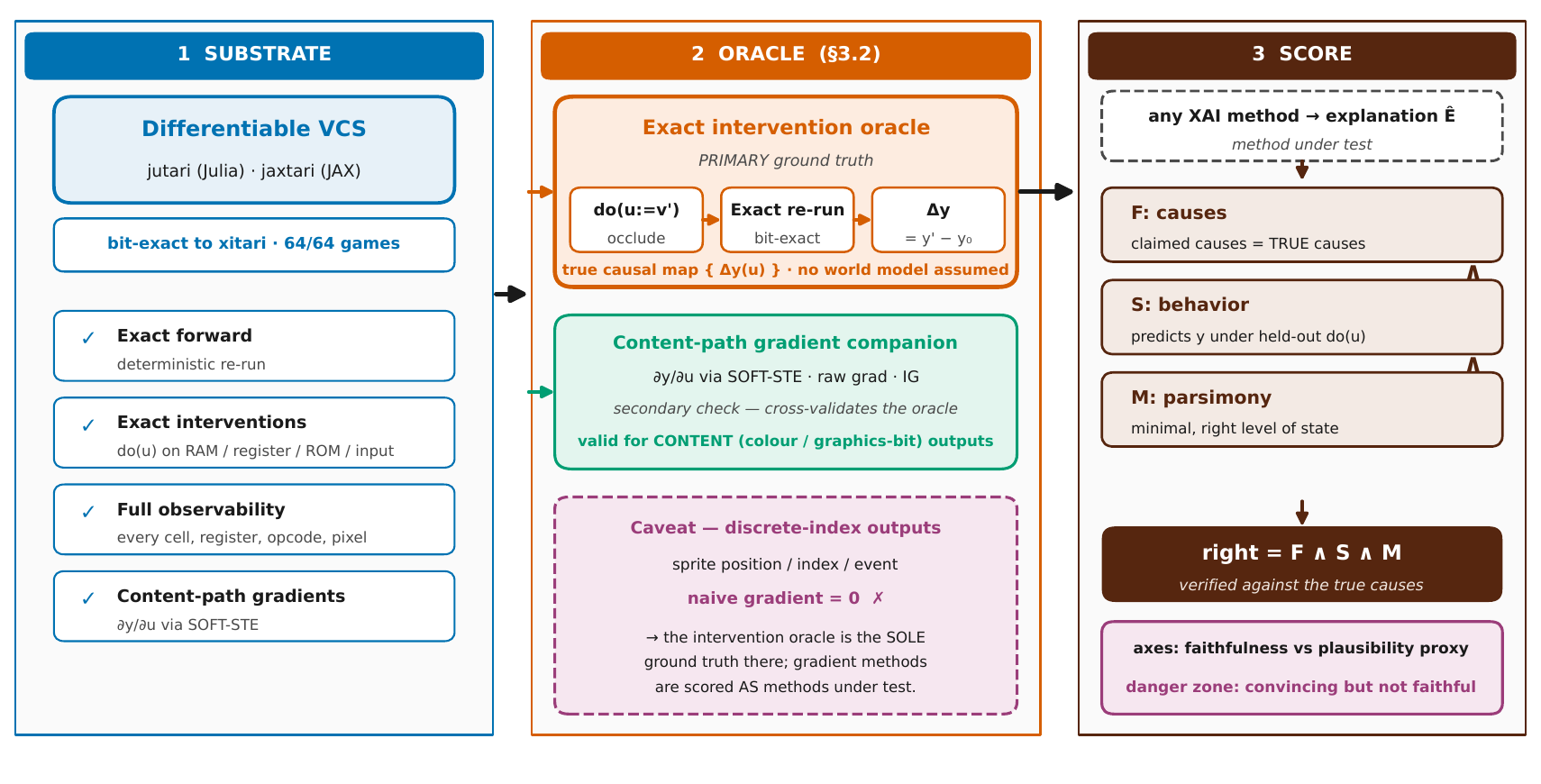
Paper 2, Fig. 1: the platform and the intervention oracle.
4 · The oracle: ground truth by intervention
Causality has a precise meaning (causal models, do-calculus): \(u\) causes \(y\) if setting \(u\) to another value, with everything else held fixed, changes \(y\). Observing that \(u\) and \(y\) move together is not enough. On a network this experiment is expensive and ambiguous. On a deterministic, bit-exact emulator it is trivial:
- Reach a state. Boot the game and play 90 frames of seeded random joystick input
shared_testbed_impl.jl:71. Save the machine at that frame, \(f^*\) (the checkpoint)shared_testbed_impl.jl:115. - Define causes. For each RAM byte that the community annotations (AtariARI, OCAtari)
say means something, such as a ball x-position or a score, make two interventions: set it to
its value +17, and zero it. Add a TIA colour register and a different joystick action
oracle_intervene.jl:185. - Intervene and re-run. For each cause: copy the checkpoint, poke the value
jutari_oracle.jl:176, play the same 15 frames, read the outputoracle_intervene.jl:242. - Measure. The true effect is \(|\Delta y(u)| = |y(do(u)) - y(\text{baseline})|\)
saliency.jl:301. Every number is a real re-run, with no approximation.
Every state is checked by a cause-density gate: at least four causes must actually move the screen output, and each record notes whether its state passed, so a state where nothing happens is flagged rather than silently scored.
5 · How a method is scored
A method produces one score per cause, \(a(u)\). We compare it with the oracle \(|\Delta y(u)|\):
- Pearson and Spearman correlation
pilot_ig_vs_oracle.jl:173: do big attributions go with big true effects? - Precision@3
pilot_ig_vs_oracle.jl:198: of the method's top-3 causes, how many are in the oracle's top-3? - Deletion / insertion curves
saliency.jl:264: apply the causes in the method's order on the real machine and watch the output move. A good ranking moves it early. - Positive control: the oracle itself, scored as if it were a method, must come out perfect. This proves the harness is not broken.
These roll up into the paper's triad. Faithful: agrees with the oracle. Sufficient: predicts held-out interventions. Minimal: names no more causes than necessary. An explanation is only “correct” if it is all three. The leaderboard shows where each method lands.
6 · Two outputs, two lessons
Content outputs (a stored value) flow through arithmetic the gradient can follow. Here
gradient methods have a fair chance. Position outputs depend on timing: the sprite is
drawn where the CPU happened to be when it strobed a register. A tiny change in a position byte moves
the sprite by zero pixels, until it jumps by a whole pixel. The derivative is zero almost everywhere,
which is the textbook vanishing gradient. The site reports that honest zero and, next to it, a
gradient through a differentiable bilinear sampler shared_testbed_impl.jl:357 that draws the sprite at a continuous
column, the trick used by spatial-transformer networks. Comparing the two shows how much an
attribution depends on a modelling choice the user rarely sees.
Most gradient runners differentiate the output read at \(f^*\). The
end-to-end arm e2e_gradient.jl:165 instead backpropagates from frame \(f^*{+}15\)
through every one of the ≈105 CPU instructions in between: the real “deep
network” case. The measured answer is a lesson in itself: in all 44 scored games the forward
pass stays bit-exact, yet on most of them the gradient that comes out is the same one-hot spike the
one-line read gives. Every other causal path runs through a branch, a table look-up or a hardware
read, and a gradient cannot see any of those. On 8 games the content gradient and on 8 the position
gradient dies completely on the way back (Breakout and Space Invaders among them). Only Centipede,
where the output byte is carried over from the oracle's strongest cause, gets a better map.
7 · The methods, in a suggested reading order
Each page has the same structure: the idea in plain words, how it works on a neural network (with a toy example), the translation to the VCS, the exact lines of code (method and emulator), pitfalls, and a command to reproduce it.
1 · Gradient methods — “how sensitive is the output?”
Differentiate the output with respect to the input. One backward pass, no re-runs. They need a differentiable model, which is why the VCS has a differentiable twin. Start with saliency; every other member fixes one of its problems (scale, noise, saturation, the choice of baseline).
- Vanilla gradient (saliency) — Gradient family · the starting point
- Grad×Input / DeepLIFT — Gradient family · saliency weighted by the input
- SmoothGrad — Gradient family · saliency averaged over noise
- Guided Backprop — Gradient family · a modified backward pass
- Integrated Gradients — Gradient family · path integral from a baseline
- Expected Gradients — Gradient family · Integrated Gradients averaged over baselines
2 · Perturbation methods — “what happens if I change it?”
Treat the model as a black box: change inputs, re-run, watch the output. No gradients needed. On the VCS, re-running the model means re-running the real emulator, so these are the closest relatives of the oracle. They differ in what they change and how they summarise it.
- Occlusion — Perturbation family · the starting point
- Extremal / meaningful perturbation — Perturbation family · optimise the mask
- RISE — Perturbation family · random joint masks
- LIME — Perturbation family · fit a local surrogate
- KernelSHAP / Shapley — Perturbation family · fair shares from game theory
- On-distribution counterfactual — Perturbation family · the smallest change that flips the outcome
3 · Mechanistic interpretability — “which internal parts compute it?”
Open the box. Patch internal activations between two runs, find circuits, learn feature dictionaries, probe for information. Developed for transformers and LLMs; here the “activations” are RAM bytes and registers of a machine whose circuit we can read off the ROM.
- Activation patching / causal mediation — Mechanistic family · the core causal tool
- Attribution / edge patching — Mechanistic family · patching at gradient cost
- Path patching / IOI circuit — Mechanistic family · patching the wiring, not the nodes
- ACDC — automatic circuit discovery — Mechanistic family · circuit discovery, automated
- Interchange interventions / DAS — Mechanistic family · testing a hypothesis about a variable
- Causal scrubbing — Mechanistic family · testing a circuit hypothesis
- Sparse autoencoders — Mechanistic family · features from superposition
- NMF/PCA dictionaries — Mechanistic family · classical dictionary learning
- Linear probing + control tasks — Mechanistic family · decoding what is represented
- Logit / tuned lens — Mechanistic family · reading intermediate states
4 · The neuroscience battery — “could a neuroscientist understand a microprocessor?”
The classic toolbox of systems neuroscience — lesions, tuning curves, correlations, field potentials, Granger causality, dimensionality reduction — applied to a chip, after Jonas & Kording (2017). Many of these have direct deep-learning analogues (ablations, neuron selectivity, PCA of activations).
- A1 · Connectomics / data-flow graph — Phase A · neuroscience battery · wiring from perturbation
- A2 · Single-unit lesions — Phase A · neuroscience battery · knock one unit out
- A3 · Tuning curves — Phase A · neuroscience battery · what does this unit respond to?
- A4 · Pairwise correlations — Phase A · neuroscience battery · who fires together?
- A5 · Local field potentials — Neuroscience battery · pooled signals and their rhythms
- A6 · Granger causality — Neuroscience battery · causal discovery from timing alone
- A7 · Dimensionality reduction (NMF/PCA) — Neuroscience battery · latent factors of population activity
- A8 · Whole-state recording — Neuroscience battery · the record-everything baseline
5 · When a method does not apply
Some methods assume things the VCS does not have (e.g. attention heads, a token vocabulary). Marking them not-applicable, with the reason, is part of an honest benchmark.
- N/A audit: Grad-CAM, attention rollout, VIPER — Applicability audit · what a method needs before it can run
8 · Glossary
| Attribution | A score per input (or per internal unit) saying how much it contributed to an output. |
|---|---|
| Faithfulness (F) | Does the explanation agree with what the model actually does? Here: correlation of the method's scores with the oracle's true effects. |
| Sufficiency (S) | Can the explanation predict what happens under new, held-out interventions? |
| Minimality (M) | Does the explanation name only what is needed? True minimal cause set / named set. |
| Intervention / do(·) | Setting a variable to a value by force and re-running, as opposed to merely observing it. Written \(do(u := v)\). |
| Oracle | Here: the exact answer to “what does intervention \(u\) do to output \(y\)?”, obtained by actually re-running the bit-exact emulator. |
| Cause \(u\) | One candidate intervention: a RAM byte set to a new value or zeroed, a TIA colour register, or a different joystick action. |
| Content output | A value the machine stores (one RAM byte at the end of the horizon), e.g. the score. |
| Position output | How many screen pixels differ from the un-intervened frame: depends on where a sprite is drawn. |
| Vanishing gradient | A gradient that is exactly zero although the input matters, because the function is flat or piecewise constant around the current point. |
| Straight-through estimator (STE) | Use the exact (hard, discrete) value in the forward pass and a smooth surrogate's derivative in the backward pass. |
| Bit-exact | Every RAM byte, register and pixel identical to the reference emulator (xitari / the Arcade Learning Environment) at every frame. |
| Frame | One video picture: 262 scanlines, about 1/60 s, a few thousand CPU instructions. |
| Horizon | The number of frames played after the intervention before the output is read (15 here). |
| Baseline / reference | The “neutral” input some methods compare against (Integrated Gradients, SHAP, occlusion). Choosing it is a modelling decision, not a detail. |
| Superposition | A network storing more features than it has neurons, by overlapping them; the reason sparse autoencoders are used. |
9 · Run it yourself
git clone https://github.com/akmaier/UnderstandingVCS
cd UnderstandingVCS
julia --project=jutari -e 'using Pkg; Pkg.instantiate(); Pkg.test()'   # emulator self-test, ~20 s
julia --project=jutari tools/xai_study/phaseB_attribution/saliency.jl --game pong
The ROMs are not in the repository (licence). See Reproduce for how to obtain them and verify their SHA-256 hashes.