Phase A · neuroscience battery

A1 · Connectomics / data-flow graph

cf. Jonas & Kording 2017

← back to the method catalogue

What it does?

Connectomics tries to map the wiring of a system by watching how its parts affect each other. In neuroscience it means reconstructing which neurons connect to which. Here we do the same for the machine's memory. We change one RAM cell, re-run the program, and record which other cells change as a result. Each such dependency is drawn as a directed edge from cause to effect. The full set of edges is the program's data-flow graph, its 'connectome'. The idea is that the pattern of who-influences-whom should reveal the computation, without reading the code. This is a classic move in systems neuroscience: infer function from structure. On the VCS we have the true wiring from the disassembly, so we can check whether the recovered graph is right. The method is attractive because it needs no labels and no model of what the program means. It only needs the ability to perturb and observe. In practice it recovers a graph that looks plausible but contains many edges the real program does not have, because a single perturbation ripples through shared clocks and buffers.

A1 · Connectomics / data-flow graph result

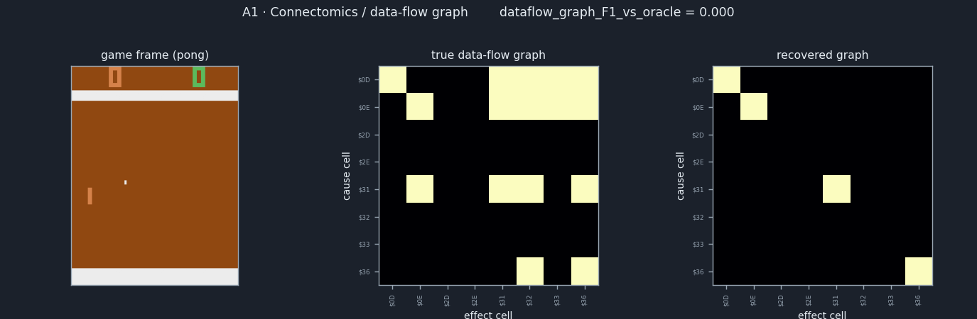
Two adjacency matrices over the candidate RAM cells: the true data-flow graph and the graph this method recovered. A bright cell (row = cause, column = effect) is an edge; the difference between the two panels is the error. dataflow_graph_F1_vs_oracle = 0.000 — this example only (pong, state gameplay(seed=0,prefix=90)+15); the audit aggregate is below.

How it's scored

The score is a data-flow-graph F1 against the true read/write graph from the disassembly. An edge means that perturbing one RAM cell changes another. We build the recovered graph by single-shot perturbation and compare its edges to the true edges, taking the harmonic mean of precision, the fraction of recovered edges that are real, and recall, the fraction of real edges recovered. Faithfulness for this method is that edge F1: a graph-valued explanation is graded as a graph, not as a heat-map. The comparison is always against the intervention oracle's true wiring, never against another method. The hard part is that a single perturbation ripples through shared clocks and buffers, so the recovered graph contains many edges the real program does not have. Precision suffers, and the F1 stays low. There is no separate position hard-case here, because the method never claims a sprite position; it claims a wiring diagram. The audit box below reports the actual F1, aggregated across the scored games, so no single game dominates. Read the recovered-versus-true graph as the error: every edge in one panel but not the other is a mistake the metric counts.

The score is measured against the §1 intervention oracle — never against another interpretability method. F (faithful) is always vs the oracle; see the execution stack. How each of F / S / M is actually computed for this method (and whether it matches the paper) is in the box just below; the numbers are in the In the audit box under it.

How F, S, M are computed here

The exact formula this method uses for each score, read from its runner, and whether it matches the paper's §3 (F ∧ S ∧ M triad) definition. From the committed audit fsm_math_phaseA.json.

AxisFormula (as computed) What it measuresMatches §3?
F
faithfulness
\(F = F_1^{\mathrm{edge}}(\hat{E}, E^{\star})\)F1 of the single-shot recovered data-flow edges against the exact-oracle true data-flow graph over 8 candidate cells.✓ matches Graph-valued primitive = edge F1 vs true data-flow graph, exactly the paper's connectomics case. Runner A1_connectomics.jl,; record out/A1_pong.json extra.triad.F=0.0 / graph.f1.
how it's measured — call stack:
  1. F = edge-F1 of the recovered do(base+17) edges vs the true graph — A1_connectomics.jl:406
  2. score_graph: edge precision, recall and F1 of the two graphs — A1_connectomics.jl:367
  3. true causal effect Δy(u) by bit-exact re-run — oracle_intervene.jl:242
S
sufficiency
\(S = \dfrac{\#\{(i,j):\ \hat{E}_{ij}=E^{\star,\mathrm{held}}_{ij}\}}{\#\,\mathrm{off\text{-}diag}} \in [0,1]\)Off-diagonal edge agreement between the base+17 recovered graph and the held-out base+37 true edge set (unseen intervention value).✓ matches Held-out edge agreement between the base+17 recovered graph and the held-out base+37 true edge set: a non-null held-out sufficiency. §3 (sec:triad) admits the fraction-within-tolerance [0,1] special case of the held-out predictive test, which this off-diagonal edge-agreement fraction satisfies. A1_connectomics.jl,; record S=0.839.
how it's measured — call stack:
  1. S = off-diagonal edge agreement, recovered vs held-out true edges — A1_connectomics.jl:416
  2. heldout_true_graph: true edges under the unseen do(base+37) — A1_connectomics.jl:578
M
minimality
\(M = |U^{\star}| / |\hat{U}| = |E^{\star}| / |\hat{E}| \in (0,1]\)True-graph edge count over the number of recovered edges (edge-level |U*|/|U_hat|).✓ matches Runner now emits M = |U*|/|U_hat| over edges (M_note '|true edges|=12 / |discovered edges|=0'); the paper's minimality ratio applied at the edge level. Record out/A1_pong.json extra.triad.M (null in pong when 0 edges discovered). Replaced the former 1 − FP-rate (edge precision).
how it's measured — call stack:
  1. M = |true edges| / |discovered edges| — A1_connectomics.jl:422
  2. score_graph counts the true and recovered edge sets — A1_connectomics.jl:367

✓ matches = the same quantity as §3; ◐ partial = the same kind of estimator but a differing detail; ✗ does not match = a different quantity (see the note). Definitions: F = agreement with the oracle's true causal effects Δy(u); S = held-out predictive score in [−1, 1]; M = |U*|/|Û| (true-minimal-set size / named-set size).

In the audit

This is the method's entry in the actual cross-method audit — scored on the paper's correctness triad, each axis a mean over all 35 scored games (35 committed §R records), not the single example shown above. Tradition: intervention. The example figure (Pong) is one of those records.

0.207F — faithfulness vs oracle (mean over 35 games, ±0.084 CI95)
0.971S — sufficiency: held-out predictive (n/a where the paper does not define this axis)
0.967M — minimality: true-minimal-set / named-set (n/a otherwise)
35committed records aggregated
0.00human-plausibility proxy

F faithfulness (scored vs the oracle for every method) · S sufficiency (held-out predictive score in [−1, 1]; a negative value means the explanation predicts held-out interventions worse than the unperturbed baseline; reported for the predictive methods across all three phases where the calibration/held-out split is defined) · M minimality (true-minimal-set / named-set; where the method names a cause set) — n/a otherwise, per the paper's F ∧ S ∧ M triad.

Source: leaderboard.json · the whole leaderboard is on the methods page and the Paper 2 audit.
Results per game

This method's faithfulness on each of the 35 scored games (all-regime F; this method has no content-vs-position split (see the note below)). Click a header to sort. Every number is read from site_data.json (methods.A1_connectomics.per_game).

content-F and position-F are n/a for this method. The content-vs-position split applies only to pixel-attribution methods — those that produce an attribution map over the framebuffer, whose score can be read separately on the smooth content outputs and the discrete position outputs (where the naive gradient is provably zero). This method does not attribute to a pixel output; it is graded by its own fidelity metric (dataflow_graph_F1_vs_oracle), reported as the F column, so there is no content or position regime to separate.

M is n/a on 15 of these games. Minimality is M = |U*|/|Û|, the size of the true minimal cause set over the size of the set the method actually names. On a game where the method names nothing (|Û| = 0 — it discovers no circuit, its attribution map is all-zero, or it decodes no cell), that ratio is undefined, so M is left blank rather than scored. The aggregate M is the mean over the 20 games where the method did name a cause set.

GameF (all)content-Fposition-FSMNote
Q*bert1.000n/an/a1.0001.000recovers the true causes
Bowling0.667n/an/a1.0001.000
Video Pinball0.667n/an/a0.9761.000
Tennis0.533n/an/a0.9671.000
Space Invaders0.500n/an/a0.9821.000
Chopper Command0.452n/an/a0.9901.000
Road Runner0.444n/an/a0.9871.000
Hero0.400n/an/a0.9891.000
Private Eye0.364n/an/a1.0001.000
Krull0.333n/an/a0.9750.333
Riverraid0.320n/an/a0.9721.000
Pitfall0.308n/an/a0.9751.000
Breakout0.286n/an/a1.0001.000
Seaquest0.250n/an/a0.9841.000
Carnival0.200n/an/a0.9971.000
Double Dunk0.125n/an/a0.9011.000
Montezuma's Revenge0.125n/an/a0.9761.000
Boxing0.111n/an/a0.8911.000
Demon Attack0.105n/an/a0.9621.000
Berzerk0.043n/an/a0.9571.000no true-cause signal
Air Raid0.000n/an/a0.987n/ano true-cause signal
Alien0.000n/an/a1.000n/ano true-cause signal
Assault0.000n/an/a0.990n/ano true-cause signal
Atlantis0.000n/an/a1.000n/ano true-cause signal
Centipede0.000n/an/a0.972n/ano true-cause signal
Frostbite0.000n/an/a0.977n/ano true-cause signal
Ice Hockey0.000n/an/a0.922n/ano true-cause signal
Jamesbond0.000n/an/a0.981n/ano true-cause signal
Kangaroo0.000n/an/a0.995n/ano true-cause signal
Ms. Pac-Man0.000n/an/a0.947n/ano true-cause signal
Pacman0.000n/an/a0.982n/ano true-cause signal
Phoenix0.000n/an/a0.992n/ano true-cause signal
Pong0.000n/an/a0.839n/ano true-cause signal
Venture0.000n/an/a0.938n/ano true-cause signal
Yars' Revenge0.000n/an/a0.974n/ano true-cause signal

Call stack — how it runs on jutari / jaxtari

The path from this method's runner (run_game) into the bit-exact VCS substrate, and the computation it involves. Every step links to the exact source on main. From callstack_phaseA.json.

Applied on the substrate

  1. assemble the shared gameplay-state testbed (seeded random-action stream, bit-exact checkpoint at f*, cause-density gate) — build_a1_shared_state(game) -> build_shared_testbed(game; ...) runner
  2. build_shared_testbed definition: booted checkpoint + shared n_changed_px output + cause-density gate — function build_shared_testbed(game; ...) runner
  3. cause-density gate scores each cause via the injected oracle run_intervention and counts |Delta_y|>floor — cause_density = count(>(floor), deltas) runner
  4. boot the real ROM and deterministically replay to the intervention frame (runner-local boot_replay) — checkpoint = boot_replay(spec, actions, target_frame) runner
  5. fresh env with xitari-parity boot (60 NOOP + 4 RESET) inside boot_replay — env_reset!(env; boot_noop_steps=60, boot_reset_steps=4) runner
  6. step the real emulator one frame per action — env_step!(env, Int(actions[i])) jutari
  7. read the 128-byte RIOT RAM out of the console — get_ram(env) jutari
  8. snapshot RAM+screen at the target frame (state to run the graph on) — at_target = continue_from(checkpoint, Int[]) runner

The computation

  1. the RECOVERED data-flow graph (method under test): single cheap do(i:=base+17), 1-step latency, edge i->j iff cell j differs from baseline — recovered_dataflow_graph(checkpoint, tail, cands, at_target; delta=17, latency=1) runner
  2. the TRUE data-flow graph (ground truth): exhaustive do-set {0, base+17, base+37} at full horizon, edge i->j iff cell j changes for ANY value — true_dataflow_graph(checkpoint, tail, cands, at_target) runner
  3. each edge probe intervenes on a RAM byte then re-runs the tail (uses intervene_ram!) — intervene_continue(checkpoint, c.ram_index, v, tail) runner
  4. score recovered vs true adjacency: precision/recall/F1/graph-edit-distance over off-diagonal edges — score_graph(rec_graph, true_graph) runner

Scored against the exact intervention oracle Δy(u): run_intervention(checkpoint, actions, target_frame, horizon, cause).

Implementation
tools/xai_study/phaseA_kording/A1_connectomics.jl
Reference
cf. Jonas & Kording 2017
Record
A1_pong.json
All records
phaseA_kording/out

The figure is generated from the committed record by docs/gen_method_figures.py; the game frame and each RAM cell's screen footprint are produced by render_scenes.jl / cell_footprints.jl.